A practical look at latency in robotics: The importance of metrics and operating systems

Latency is an important practical concern in the robotics world that is often poorly understood. I feel that a better understanding of latency can help robotics researchers and engineers make design and architecture decisions that greatly streamline and accelerate the R&D process. I’ve personally spent many hours looking for information on the latency characteristics of various robotic components but have had difficulty finding anything that is clearly presented or backed by solid data. From what I’ve found, most benchmarks focus on the maximum throughput and either ignore the subject of latency or measure it incorrectly.

Because of this my first post is on the topic of latency and will cover two main topics:

• The details of how you measure latency matters.
• The OS that you use affects your latency.

Over the course of several years of applied robotics research, we have come to believe that robotics research can be greatly accelerated by designing systems that relax hard real-time requirements on the software that is exposed to users. One approach is to implement low-level control (motor control and safety features) in dedicated components that are decoupled from high-level control (position, velocity, torque, etc.). In many cases, this can enable users to leverage common consumer hardware and software tools that can accelerate development.

For example, the Biorobotics lab at Carnegie Mellon has researchers that tend to be mechanical or electrical engineers, rather than computer scientists or software engineers. As such tend they to be less familiar with Linux and C/C++ and much more comfortable with Windows/macOS and scripting languages like MATLAB. After our lab started providing cross-platform support and bindings for MATLAB (in ~2011), we ended up seeing a significant increase in our research output that roughly doubled the lab’s paper publications related to snake robots. In particular, the lab has been able to develop and demonstrate new complex behaviors that would have been difficult to prototype beforehand (see compliant control or inside pipes).

Measuring latency

Robots are controlled in real-time, which means that a command gets executed within a deadline (fixed period of time). There are hard real-time systems that must never exceed their deadline, and soft real-time systems that are able to occasionally exceed their deadline. Missing deadlines when performing motor control of a robot can result in unwanted motions and ‘jerky’ behavior.

Although there is a lot of information on the theoretical definition of these terms, it can be challenging to determine the maximum deadline (point at which a system’s performance starts to degrade or become unsafe) for practical applications. This is especially true for research institutions that build novel mechanisms and target cutting-edge applications. Many research groups end up assuming that everything needs to be hard real-time with very stringent deadlines. While this approach provides solid performance guarantees, it can also create a lot of unnecessary development overhead.

Many benchmarks and tools make the assumption that latency follows a Gaussian distribution and report only the mean and the standard deviation. Unfortunately, latency tends to be very multi-modal and the most important part of the distribution when it comes to determinism are the ‘outliers’. Even if a system’s latency behaves as expected in 99% of the cases, the leftover 1% can be worse than all of the other 99% of measurements combined. Looking at only the mean and standard deviation completely fails to capture the more systemic issues. For example, I’ve seen many data sets where the worst observed case was more than 1000 standard deviations away from the mean. Such stutters are usually the main problem when working on real robotic systems.

Because of this, a more appropriate way to look at latency is via histograms and percentile plots, e.g.,“99.9% of measurements were below X ms”. There are several good resources about recording latency out there that I recommend checking out, such as How NOT to Measure Latency or HdrHistogram: A better latency capture method.

Operating systems

The operating system is at the base of everything. No matter how performant the high-level software stack is, the system is fundamentally bound by the capabilities of the OS, it’s scheduler, and the overall load on the system. Before you start optimizing your own software, you should make sure that your goal is actually achievable on the underlying platform.

There are trade-offs between always responding in a timely manner and overall performance, battery life, as well as several other concerns. Because of this, the major consumer operating systems don’t guarantee to meet hard deadlines and can theoretically have arbitrarily long pauses.

However, since using operating systems that users are familiar with can significantly ease development, it is worth evaluating their actual performance and capabilities. Even though there may not be any theoretical guarantees, the practical differences are often not noticeable.

Developing hard real-time systems has a lot of pitfalls and can require a lot of development effort. Requiring researchers to write hard real-time compliant code is not something that I would recommend.

Benchmark Setup

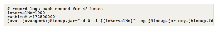
Azul Systems sells products targeted at latency sensitive applications and they’ve created a variety of useful tools to measure latency. jHiccup is a tool that measures and records system level latency spikes, which they call ‘hiccups’. It measures the time for sleep(1ms) and records the delta to the fastest previously recorded sample. For example, if the fastest sample was 1ms, but it took 3ms to wake up, it will record a 2ms hiccup. Hiccups can be caused by a large number of reasons, including scheduling, paging, indexing, and many more. By running it on an otherwise idle system, we can get an idea of the behavior of the underlying platform. It can be started with the following command:

Windows / Mac / Linux

Let’s first look at the performance of consumer operating systems: Windows, Mac and Linux. Each test started off with a clean install for each OS. The only two modifications to the stock installation were to disable sleep mode and to install JDK8 (update 101). I then started jHiccup, unplugged all external cables and let the computer sit ‘idle’ for >24 hours. The actual OS versions were,

• Windows 10 Enterprise, version 1511 (OS build: 10586.545)
• OS X, version 10.9.5
• Ubuntu 16.04 Desktop, kernel 4.4.0-31-generic

Each image below contains two charts. The top section shows the worst hiccup that occured within a given interval window, i.e., the first data point shows the worst hiccup within the first 3 minutes and the next data point shows the worst hiccup within the next 3 minutes. The bottom chart shows the percentiles of all measurements across the entire duration. Each 24 hour data set contains roughly 70-80 million samples.

Figure 1. Windows vs. Linux vs. Mac hiccups (24h)

These results show that Linux had fewer and lower outliers than Windows. Up to the 90th percentile all three systems respond relatively similarly, but there are significant differences at the higher percentiles. There also seems to have been a period of increased system activity on OSX after 7 hours. The chart below shows a zoomed in view of a 10 minute time period starting at 10 hours.

Figure 2. Windows vs. Linux vs. Mac hiccups (10min)

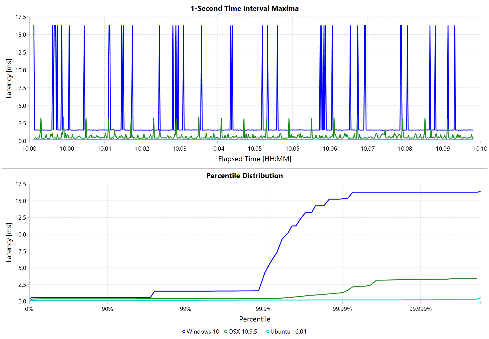
Zoomed in we can see that the Windows hiccups are actually very repeatable. 99.9% are below 2ms, but there are frequent spikes to relatively discrete values up to 16ms. This also highlights the importance of looking at the details of the latency distribution. In other data sets that I’ve seen, it is rare for the worst case to be equal to the 99.99% percentile. It’s also interesting that the distribution for 10 minutes looks identical to the 24 hour chart. OSX shows similar behavior, but with lower spikes. Ubuntu 16.04 is comparatively quiet.

It’s debatable whether this makes any difference for robotic systems in practice. All of the systems I’ve worked with either had hard real-time requirements below 1ms, in which case none of these OS would be sufficient, or they were soft real-time systems that could handle occasional hiccups to 25 or even 100 ms. I have yet to see one of our robotic systems perform perceivably worse on Windows versus Linux.

Real Time Linux

Now that we have an understanding of how traditional systems without tuning perform, let’s take a look at the performance of Linux with a real-time kernel. The rt kernel (PREEMPT_RT patch) can preempt lower priority tasks, which results in worse overall performance, but more deterministic behavior with respect to latency.

I chose Scientific Linux 6 because of its support for Red Hat® Enterprise MRG Realtime®. You can download the ISO and find instructions for installing MRG Realtime here. The version I’ve tested was,

• Scientific Linux 6.6, kernel 3.10.0-327.rt56.194.el6rt.x86_64

Note that there is a huge number of tuning options that may improve the performance of your application. There are various tuning guides that can provide more information, e.g., Red Hat’s MRG Realtime Tuning Guide. I’m not very familiar with tuning systems at this level, so I’ve only applied the following small list of changes.

• /boot/grub/menu.lst ⇒ transparent_hugepage=never
• /etc/sysctl.conf ⇒ vm.swappiness=0
• /etc/inittab ⇒ id:3:initdefault (no GUI)
• chkconfig –level 0123456 cpuspeed off

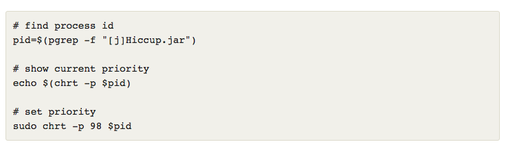
The process priority was set to 98, which is the highest priority available for real-time threads. I’d advise consulting scheduler priorities before deciding on priorities for tasks that actually use cpu time.

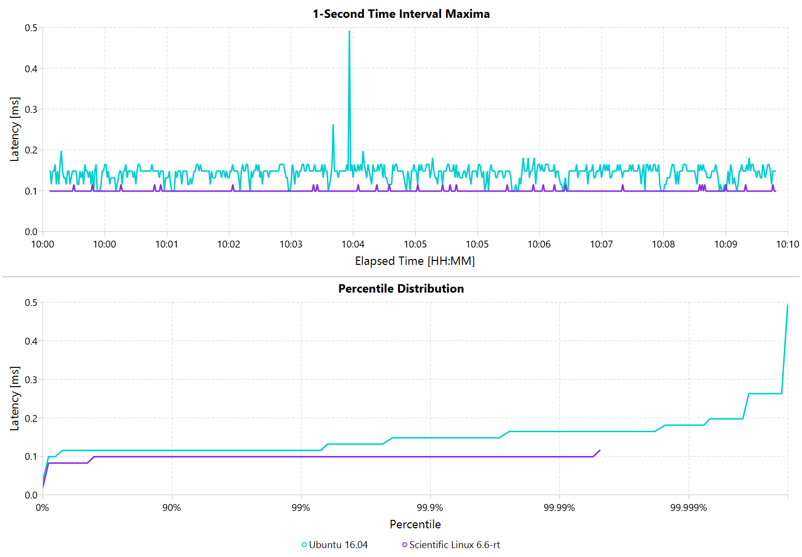
Below is a comparison of the two Linux variants.

Figure 3. Linux vs. RT Linux hiccups (24h)

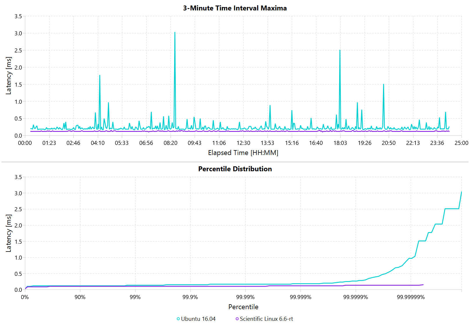
Looking at the 24 hour chart (above) and the 10 minute chart (below), we can see that worst case has gone down significantly. While Ubuntu 16.04 was barely visible when compared to Windows, it looks very noisy compared to the real-time variant. All measurements were within a 150us range, which is good enough for most applications.

Figure 4. Linux vs. RT Linux hiccups (10 min)

I’ve also added the 24-hour chart for the real-time variant by itself to provide a better scale. Note that this resolution is getting close to the resolution of what we can measure and record.

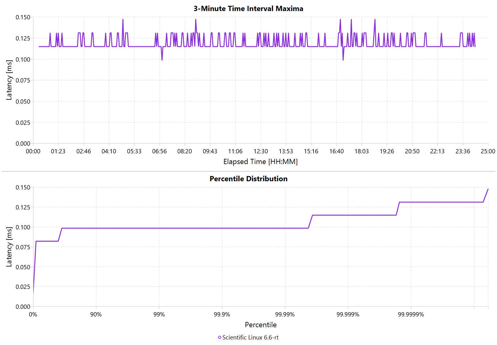
Figure 5. RT Linux hiccups (24h)

Summary

I’ve tried to provide a basic idea of the out of the box performance of various off the shelf operating systems. In my experience, the three major consumer OS can be treated relatively equal, i.e., either software will work well on all of them, or won’t work correctly on any of them. If you do work on a problem that does have hard deadlines, there are many different RTOS to choose from. Aside from the mentioned real-time Linux and the various embedded solutions, there are even real-time extensions for Windows, such as INtime or Kithara.

We’ve had very good experiences with implementing the low-level control (PID loops, motor control, safety features, etc.) on a per actuator level. That way all of the safety critical and latency sensitive pieces get handled by a dedicated RTOS and are independent of user code. The high-level controller (trajectories and multi-joint coordination) then only needs to update set targets (e.g. position/velocity/torque), which is far less sensitive to latency and doesn’t require hard real-time communications. This approach enables quick prototyping of high-level behaviors using ‘non-deterministic’ technologies, such as Windows, MATLAB and standard UDP messages.

For example, the high-level control in Teleop Taxi was done over Wi-Fi from MATLAB running on Windows, while simultaneously streaming video from an Android phone in the back of the robot. By removing the requirement for a local control computer, it only took 20-30 lines of code (see simplified, full) to run the entire demo. Actually using a local computer resulted in no perceivable benefit. While not every system can be controlled entirely through Wi-Fi, we’ve seen similar results even with more complex systems.

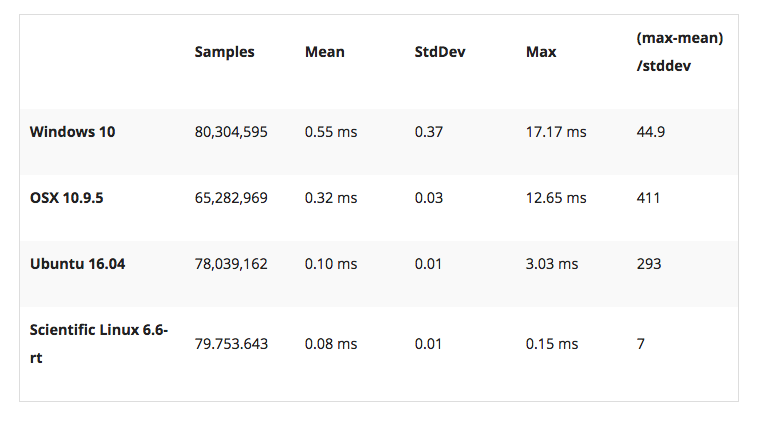
Latency is not Gaussian

Finally, I’d like to stress again that latency practically never follows a Gaussian distribution. For example, the maximum for OSX is more than 400 standard deviations away from the average. The table for these data sets is below.

The figure below compares the data’s actual distribution for Windows to a theoretical gaussian distribution. Rather than a classic ‘bell-curve’, it shows several spikes that are spread apart in regular intervals. The distance between these spikes is almost exactly one millisecond, which matches the Windows timer interrupt interval that was set while gathering the data. Interestingly, the spikes at above 2ms all seem to happen at roughly the same likelihood.

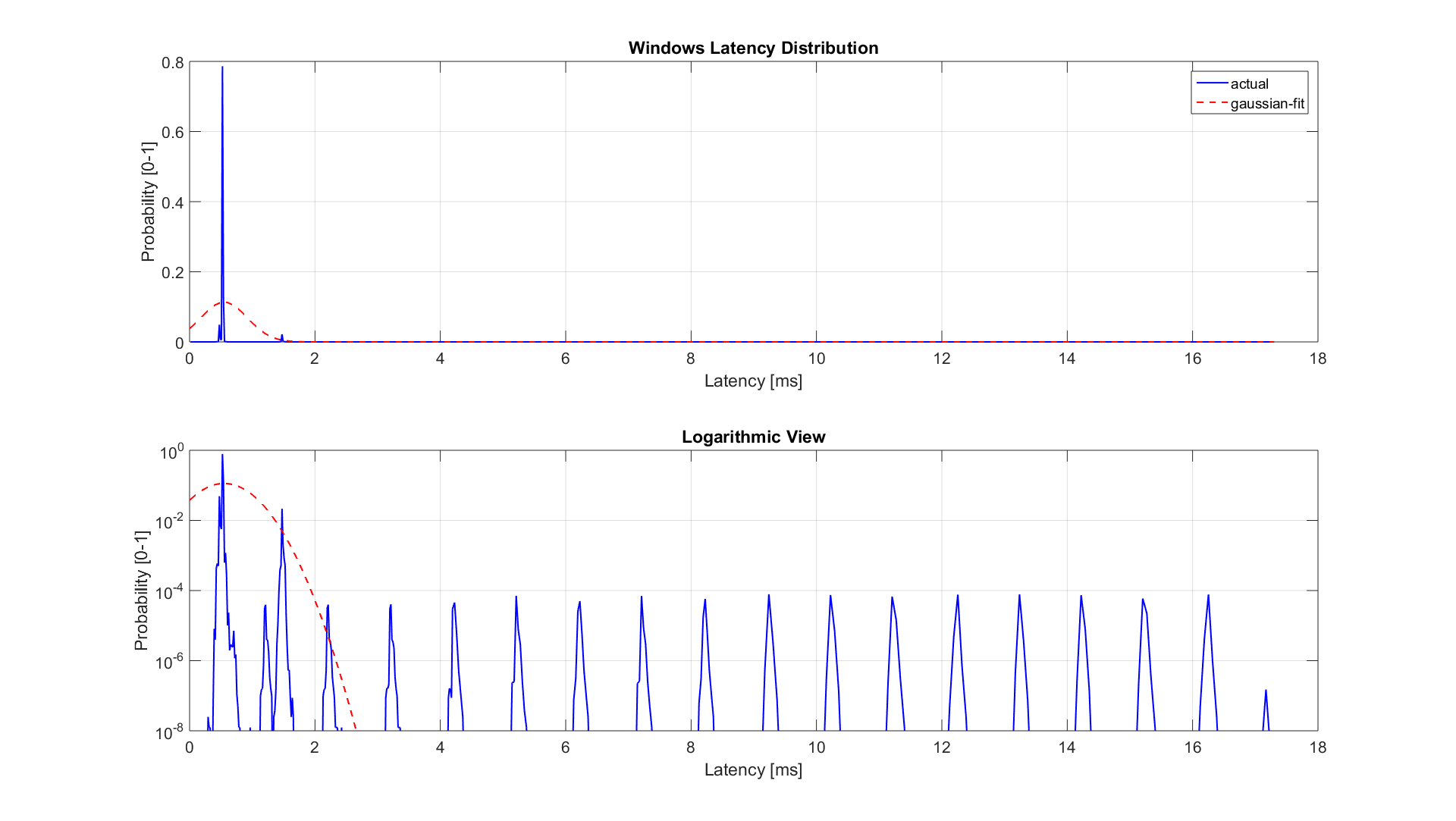
Figure 6. Actual Distribution compared to Gaussian-fit (Windows)

Using only mean and standard deviation for any sort of latency comparison can produce deceptive results. Aside from giving little to no information about the higher percentiles, there are many cases where systems with seemingly ‘better’ values exhibit worse actual performance.

The post: A Practical Look at Latency in Robotics : The Importance of Metrics and Operating Systems appeared first on Software for Robots.

Florian Enner is a Co-Founder of HEBI Robotics and a Principal Systems/Software Engineer at Carnegie Mellon University.

Florian Enner is a Co-Founder of HEBI Robotics and a Principal Systems/Software Engineer at Carnegie Mellon University.