
Robohub.org
Sample efficient evolutionary algorithm for analog circuit design
By Kourosh Hakhamaneshi
In this post, we share some recent promising results regarding the applications of Deep Learning in analog IC design. While this work targets a specific application, the proposed methods can be used in other black box optimization problems where the environment lacks a cheap/fast evaluation procedure.

So let’s break down how the analog IC design process is usually done, and then how we incorporated deep learning to ease the flow.
The intent of analog IC design is to build a physical manufacturable circuit that processes electrical signals in the analog domain, despite all sorts of noise sources that may affect the fidelity of signals. Usually analog circuit design starts off with topology selection. Generically speaking, engineers usually come up with topology of certain blocks and try to size them such that after putting them together the entire system behaves in a certain way and satisfies some figures of merit. There are certain levels of simulations and tests that need to take place to verify that the system will work before manufacturing. At the lowest level engineers do their design using their intuition and equations and then simulate and make the corresponding changes until they converge to a working design. The more accurate the simulation, the more time it takes to run. Unfortunately, in recent advanced technologies the large disparity between post-layout simulation (physical realization of the circuit) and schematic simulation (circuit concept) requires designers to be aware of the parasitic effects due to the way the circuit is physically implemented. This basically means that simulations take longer, and on top of that more manual iterations are needed.
Now that we understand the environment let’s give a brief overview of past attempts to automate some parts of this process.
Historically people have tried different degrees of automation in different parts of the design flow (a complete ancient survey can be found in this textbook, and more recent work includes Bayesian optimization and RL). We are mostly interested in approaches that find the optimal sizing for a given topology to satisfy a collection of metrics (a constraint satisfaction problem).
Some people have derived analytical formulations for behavior of circuits and turned the problem into optimization over these analytical expressions (for example by expressing gain as an analytical function of transistor sizes). However, as was mentioned earlier, today, even schematic simulations can differ from their layout counterpart. So those ancient approaches lost their attractiveness very early on due to this important drawback.
Some other approaches tried to use simulations and modeled the problem as a black box optimization. A lot of them showed success in simple circuits in schematic-based simulations, but again could not scale very well to larger circuits and layout exploration. The bottom line till now is that a lot of iterations are needed and long simulations make it even more difficult and cumbersome.
On a side note, population based black-box optimization algorithms achieve a pretty good performance, in terms of the final output’s quality. For example, this paper shows a setting where RL agents are trained in a parallelized fashion using scalable evolutionary algorithms. The problem is that they are insanely sample inefficient (despite being parallelizable) and their exploration strategy is mostly stochastic with no “real” guidance. The problem with circuit design is that tools available for simulation are not highly parallelizable or very expensive to parallelize. In this work we have proposed a new way to make them more sample efficient.
Let’s formalize the problem a bit. Let’s say we want to design an amplifier with a given topology for a gain larger than $A_0$ and a bandwidth larger than $BW_0$. We want to find the “optimum” sizes for the components of the circuit such that they satisfy these performance constraints. We can formulate the problem as minimizing a scalar cost function equal to the sum of relative errors to the required specification. More concretely, in this example:
And we get the $A(x)$ and $BW(x)$ values after simulation.
To state it in a more general form:
Where $x$ presents the geometric parameters in the circuit topology and
represents the normalized spec error for designs that do not satisfy constraint , or zero if they do. $c_i$ denotes the value of constraint $i$ at input $x$, and is evaluated using a simulation framework. denotes the optimal value. Intuitively this cost function is only accounting for the normalized error from the unsatisfied constraints, and $w_i$ is the tuning factor, determined by the designer, which controls prioritizing one metric over another if the design is infeasible.
In principle, we can start optimizing $cost(x)$ by using evolutionary algorithms (a great intro found here). In fact we used deap to implement a baseline version of genetic algorithm to our problem. The issue is that there is no “real” intelligence in exploration, and therefore, it takes a lot of expensive simulations to find a solution, even for the simplest design problems. To put it in perspective let’s work with a 3D contrived example, let’s say the current population includes $x_1$, $x_2$, and $x_3$ among which none satisfy all specs under consideration.
Now let’s say our chance hits and we produce the following $y$ samples from the old population.
We know the performance of $x$ samples and to know performance of $y$ samples we need to run simulations (this is the part which can potentially be extremely slow).
Now let’s say after simulation we sort samples by their performance and get the following next generation of population.
Observe that after this “unlucky” iteration $y_2$ and $y_3$ got eliminated. In our proposed method, we devised a model to predict the performance before simulation and only simulate those samples which have better predicted performance. So in our contrived example we’ll predict whether new designs have better performance than $x_1$ and if so, we simulate them. If our prediction is accurate (or almost accurate) we waste fewer simulations. On the other hand, if we do not make accurate decisions, we could either approve samples that do not show high quality after simulation or reject designs that should have been accepted.
Next we’ll describe a model that was able to achieve acceptable results utilizing this idea. All implementations details can be found in the GitHub code.
Architecture Choice for the Model
This model has to have two distinct characteristics:
-
It has to be able to express how good/bad a new, not simulated sample is compared to individuals in the current population.
-
It should be able to generalize well, given very limited number of training samples (potentially 100-300 accurate simulations). However, it should not be biased towards a specific region in space and get stuck in a local optimum.
The first potential candidate is a regression model which predicts the cost value and uses that prediction to determine whether to simulate a design. The cost function that the network tries to approximate can be a non-convex and ill-conditioned one. Thus, from a limited number of samples it is very unlikely that it would generalize well to unseen data. Moreover, the cost function captures too much information from a single scalar number, so it would be hard to train, given a small number of training points and then expect it to generalize well.
Another option is to predict the value of each metric (i.e. gain, bandwidth, etc.). While the individual metric behaviour can be smoother than the cost function, predicting the actual metric value is unnecessary, since we are simply attempting to predict whether a new design is superior to some other design. Therefore, instead of predicting metric values exactly, the model can take two designs and predict only which design performs better in each individual metric.
We know that there are certain patterns in circuit parameters that make some metrics better than others (for example upsizing all transistors make the amplifier faster but costs more power). We use those parameters as the input of our network. Moreover, by forming a model that takes in pairs of designs instead of a single design we effectively expand our training sample size (a population of size 100 has ~5000 pairs). Despite the fact that neural net’s input space is larger, in practice, training is easier.
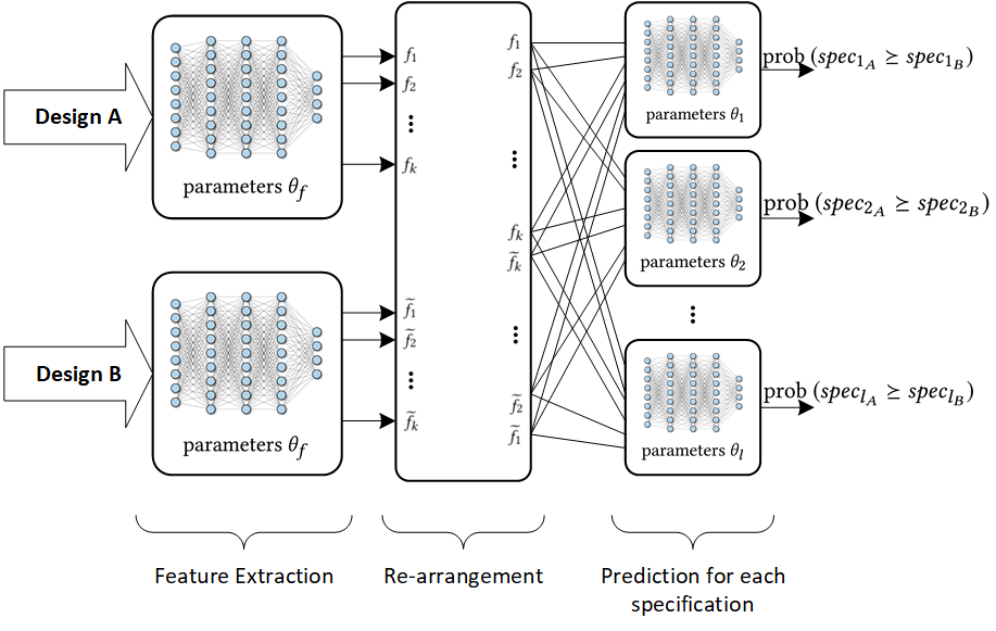
The bottom figure shows the structure of the neural net modeling the oracle simulator used in this approach. This model takes in two sets of parameters (one for Design A and one for B); extracts some useful features $(f_1, \ldots, f_k)$; rearranges the order of features (the reason for this will become clear shortly); and feeds the cascaded/rearranged feature vectors to independent neural networks to predict the superiority of Design A to Design B for a given spec. The dedicated superiority-predicting neural nets share the same architecture across all specs, but are parameterized separately. The output is interpreted as the probability that Design A is better than Design B in $\text{spec}_1$ or $\text{spec}_2$ and so on.
So during inference, the parameters of the query design are going to be fed to Design B, and the reference design to Design A. Then we predict how the query design will do compared to the reference design. Then we use some heuristic to decide whether to simulate or ignore the new design.
One other subtle constraint on the model is that there should be no contradiction in the predicted probabilities depending on the order by which the inputs were fed in. For example if we feed in A and B, and A is predicted to have a better gain than B with probability 0.8, if we swap the order of A and B the probability should become 0.2 by construction of the network. This requires a particular symmetry in the network architecture. For more info on this refer to the paper, but here is a code snippet that shows how we make sure a layer behaves like that by construction.
weight_elements = tf . get_variable ( name = 'W' , shape = [ input_data . shape [ 1 ] // 2 , layer_dim ], initializer = tf . random_normal_initializer ) bias_elements = tf . get_variable ( name = 'b' , shape = [ layer_dim // 2 ], initializer = tf . zeros_initializer ) Weight = tf . concat ([ weight_elements , weight_elements [:: - 1 , :: - 1 ]], axis = 0 , name = 'Weights' ) Bias = tf . concat ([ bias_elements , bias_elements [:: - 1 ]], axis = 0 , name = 'Bias' )
The reason that the rearrangement happens is exactly this and the code below shows how it’s actually done.
features1 = self . _feature_extraction_model ( input1_norm , name = 'feat_model' , reuse = False ) features2 = self . _feature_extraction_model ( input2_norm , name = 'feat_model' , reuse = True ) input_features = tf . concat ([ features1 , features2 [:, :: - 1 ]], axis = 1 )
To train the network, we construct all Design A and Design B permutations from the buffer of previously simulated designs and label their comparison in each metric. We then update network parameters with Adam optimizer, using sum of cross-entropy loss for all metrics.
There is also another architecture choice that helped in the overall convergence and that is using dropout layers to estimate the uncertainty in predictions. During each query, we randomly turn off 20% of the activations in each layer 5 times, and average the output probabilities to remove the uncertainty.
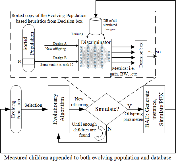
Let’s describe the figure above. Our algorithm uses some underlying evolutionary algorithm that has a broad exploration strategy. We used deap to implement our algorithm’s evolutionary strategies (code found here).
Our algorithm starts by randomly sampling the design space (for let’s say 100 designs) and simulates all of them (this part takes some time). Then the evolutionary algorithm proposes some offspring for future generations. We then use the predictive model to “guess” whether the new proposed offspring is better than some average design in the current population. So that when we really simulate, it doesn’t get eliminated.
We should keep re-training the model as more samples are added to our database; otherwise, the model gets biased to a specific region and we lose accuracy as we progress. DAgger does this for imitation learning, however the big difference here is that we can’t really re-label (simulate) rejected samples as it defeats the purpose of short run time, so we only simulate those samples which get approved by the model (either by mistake or correctly).
What’s that decision box at the output of the discriminator? That’s basically telling the prediction process, the criteria to be used for discrimination. Remember that output of model is whether a design is better than some other design in individual metrics (not overall). The decision box in summary, keeps track of the metrics we improved so far and the collection of metrics that affect the cost objective the most. For more info on details please refer to the paper, and the code.
Finally, Experiments!
We tested this methodology on a couple of circuits with different settings, gradually making the complexity more similar to today’s analog circuit design problems. The simplest relevant scenario is design of an opamp, verified in schematic (with no layout) so that simulation is cheap and we can run an oracle discriminator (based on real simulations rather than prediction of the model).
We compared that to our approach and the normal evolutionary algorithm. The details of the circuit are in the paper, but let’s look at the performance curve to prove a point here.
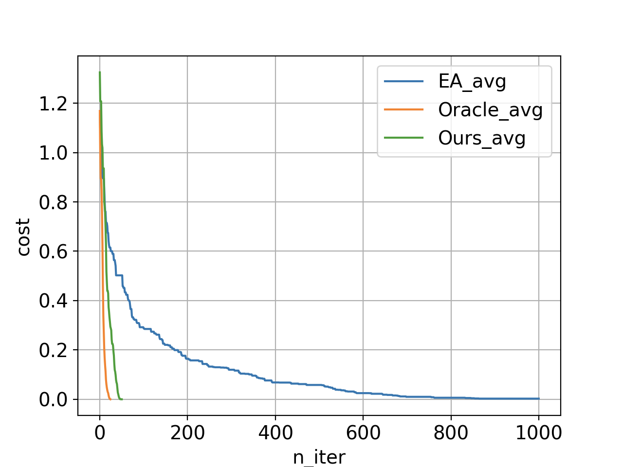
In this plot we are looking at the average cost function of the top 20 individuals in the current population as a function of number of iterations. In each iteration we simulate 5 designs and evict the worst 5 designs (to keep the evolving population size constant). If we use just the underlying evolutionary algorithm (without any discriminations) we get the blue curve (with over 5000 simulations); however, our method with neural network discrimination produces the green curve (with only 240 simulations). The orange curve shows the same method if we use the simulator the do the discriminations. Conducting the orange experiment requires simulation of all proposed samples and keeping top 5 that are actually better than design rank 20 in the current population, which means a lot of simulations (3400 simulations). The gap between the orange and green illustrates how loss of accuracy due to utilization of function approximators affects the overall optimization performance. Reaching zero means we have at least 20 designs satisfying all the specs.
We also experimented with an optical photonic receiver design – a circuit of bigger size and longer simulations – to see if this method can be applied to long post-layout simulations of designs which are more complex. In this particular example we also showed that we can even design circuits with very high level specifications. For this example the search space was of size $2.8 \times 10^{30}$ and to find the optimal designs we queried the discriminator 77487 times from which we only ran 435 simulations. This means that if we had to simulate all of them we had to wait 300x longer.
Future Directions
Evaluating the performance of the algorithm in a quantitative way is still a challenging problem. For the simple example above, we used comparisons against an oracle. However, as our circuits get bigger and more complex, running the oracle as a baseline quickly becomes unfeasible. How much certain choices in the architecture affected the total performance is an open question. We are looking into various figures of merit to account for both diversity and quality of approved samples and compare models with different choices using that.
In the results presented, we used full-accuracy post-layout simulations to optimize the system. These alterations to the circuit sizing reflected both fundamental circuit tradeoffs, as well as effects due to layout parasitics. Because schematic simulation is significantly faster than post-layout simulation, one direction for this work is to attempt to learn the circuit tradeoffs from the schematic level simulation, and then refine the models based on post-layout data.
We refer the reader to the following paper for details:
This article was initially published on the BAIR blog, and appears here with the authors’ permission.

AUAI is supported by: