
Robohub.org
Maximum Entropy RL (Provably) Solves Some Robust RL Problems
By Ben Eysenbach
Nearly all real-world applications of reinforcement learning involve some degree of shift between the training environment and the testing environment. However, prior work has observed that even small shifts in the environment cause most RL algorithms to perform markedly worse. As we aim to scale reinforcement learning algorithms and apply them in the real world, it is increasingly important to learn policies that are robust to changes in the environment.
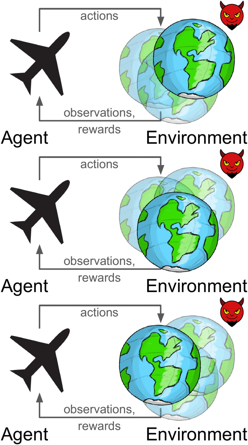
Robust reinforcement learning maximizes reward on an adversarially-chosen environment.
Broadly, prior approaches to handling distribution shift in RL aim to maximize performance in either the average case or the worst case. The first set of approaches, such as domain randomization, train a policy on a distribution of environments, and optimize the average performance of the policy on these environments. While these methods have been successfully applied to a number of areas (e.g., self-driving cars, robot locomotion and manipulation), their success rests critically on the design of the distribution of environments. Moreover, policies that do well on average are not guaranteed to get high reward on every environment. The policy that gets the highest reward on average might get very low reward on a small fraction of environments. The second set of approaches, typically referred to as robust RL, focus on the worst-case scenarios. The aim is to find a policy that gets high reward on every environment within some set. Robust RL can equivalently be viewed as a two-player game between the policy and an environment adversary. The policy tries to get high reward, while the environment adversary tries to tweak the dynamics and reward function of the environment so that the policy gets lower reward. One important property of the robust approach is that, unlike domain randomization, it is invariant to the ratio of easy and hard tasks. Whereas robust RL always evaluates a policy on the most challenging tasks, domain randomization will predict that the policy is better if it is evaluated on a distribution of environments with more easy tasks.
Prior work has suggested a number of algorithms for solving robust RL problems. Generally, these algorithms all follow the same recipe: take an existing RL algorithm and add some additional machinery on top to make it robust. For example, robust value iteration uses Q-learning as the base RL algorithm, and modifies the Bellman update by solving a convex optimization problem in the inner loop of each Bellman backup. Similarly, Pinto ‘17 uses TRPO as the base RL algorithm and periodically updates the environment based on the behavior of the current policy. These prior approaches are often difficult to implement and, even once implemented correctly, they requiring tuning of many additional hyperparameters. Might there be a simpler approach, an approach that does not require additional hyperparameters and additional lines of code to debug?
To answer this question, we are going to focus on a type of RL algorithm known as maximum entropy RL, or MaxEnt RL for short (Todorov ‘06, Rawlik ‘08, Ziebart ‘10). MaxEnt RL is a slight variant of standard RL that aims to learn a policy that gets high reward while acting as randomly as possible; formally, MaxEnt maximizes the entropy of the policy. Some prior work has observed empirically that MaxEnt RL algorithms appear to be robust to some disturbances the environment. To the best of our knowledge, no prior work has actually proven that MaxEnt RL is robust to environmental disturbances.
In a recent paper, we prove that every MaxEnt RL problem corresponds to maximizing a lower bound on a robust RL problem. Thus, when you run MaxEnt RL, you are implicitly solving a robust RL problem. Our analysis provides a theoretically-justified explanation for the empirical robustness of MaxEnt RL, and proves that MaxEnt RL is itself a robust RL algorithm. In the rest of this post, we’ll provide some intuition into why MaxEnt RL should be robust and what sort of perturbations MaxEnt RL is robust to. We’ll also show some experiments demonstrating the robustness of MaxEnt RL.
Intuition
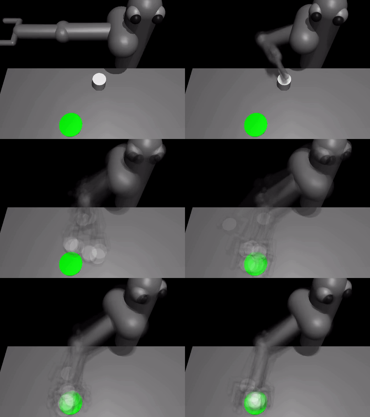
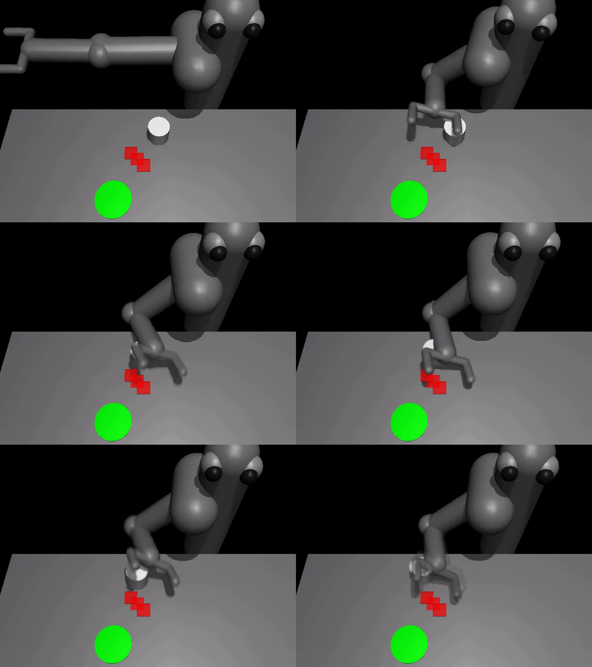
So, why would we expect MaxEnt RL to be robust to disturbances in the environment? Recall that MaxEnt RL trains policies to not only maximize reward, but to do so while acting as randomly as possible. In essence, the policy itself is injecting as much noise as possible into the environment, so it gets to “practice” recovering from disturbances. Thus, if the change in dynamics appears like just a disturbance in the original environment, our policy has already been trained on such data. Another way of viewing MaxEnt RL is as learning many different ways of solving the task (Kappen ‘05). For example, let’s look at the task shown in videos below: we want the robot to push the white object to the green region. The top two videos show that standard RL always takes the shortest path to the goal, whereas MaxEnt RL takes many different paths to the goal. Now, let’s imagine that we add a new obstacle (red blocks) that wasn’t included during training. As shown in the videos in the bottom row, the policy learned by standard RL almost always collides with the obstacle, rarely reaching the goal. In contrast, the MaxEnt RL policy often chooses routes around the obstacle, continuing to reach the goal for a large fraction of trials.
| Standard RL | MaxEnt RL | |
|
Trained and evaluated without the obstacle: |

|
|
|
Trained without the obstacle, but evaluated with |
|

|
Theory
We now formally describe the technical results from the paper. The aim here is not to provide a full proof (see the paper Appendix for that), but instead to build some intuition for what the technical results say. Our main result is that, when you apply MaxEnt RL with some reward function and some dynamics, you are actually maximizing a lower bound on the robust RL objective. To explain this result, we must first define the MaxEnt RL objective: $J_{MaxEnt}(\pi; p, r)$ is the entropy-regularized cumulative return of policy $\pi$ when evaluated using dynamics $p(s’ \mid s, a)$ and reward function $r(s, a)$. While we will train the policy using one dynamics $p$, we will evaluate the policy on a different dynamics, $\tilde{p}(s’ \mid s, a)$, chosen by the adversary. We can now formally state our main result as follows:
The left-hand-side is the robust RL objective. It says that the adversary gets to choose whichever dynamics function $\tilde{p}(s’ \mid s, a)$ makes our policy perform as poorly as possible, subject to some constraints (as specified by the set $\tilde{\mathcal{P}}$). On the right-hand-side we have the MaxEnt RL objective (note that $\log T$ is a constant, and the function $\exp(\cdots)$ is always increasing). Thus, this objective says that a policy that has a high entropy-regularized reward (right hand-side) is guaranteed to also get high reward when evaluated on an adversarially-chosen dynamics.
The most important part of this equation is the set $\tilde{\mathcal{P}}$ of dynamics that the adversary can choose from. Our analysis describes precisely how this set is constructed and shows that, if we want a policy to be robust to a larger set of disturbances, all we have to do is increase the weight on the entropy term and decrease the weight on the reward term. Intuitively, the adversary must choose dynamics that are “close” to the dynamics on which the policy was trained. For example, in the special case where the dynamics are linear-Gaussian, this set corresponds to all perturbations where the original expected next state and the perturbed expected next state have a Euclidean distance less than $\epsilon$.
More Experiments
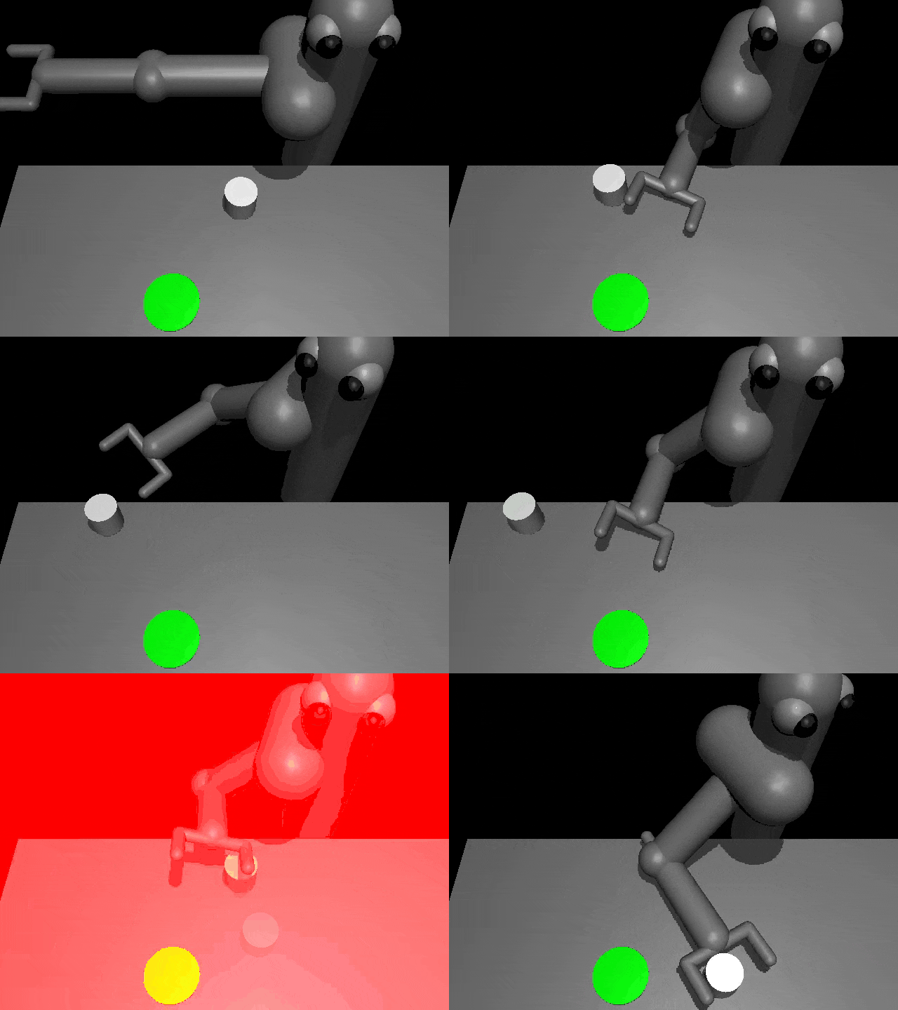
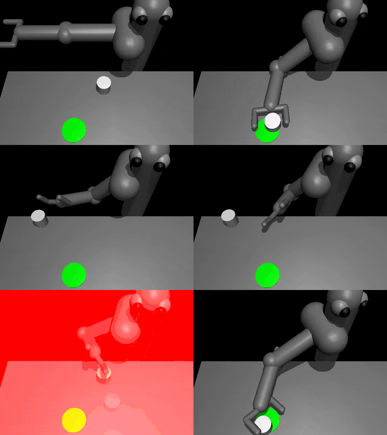
Our analysis predicts that MaxEnt RL should be robust to many types of disturbances. The first set of videos in this post showed that MaxEnt RL is robust to static obstacles. MaxEnt RL is also robust to dynamic perturbations introduced in the middle of an episode. To demonstrate this, we took the same robotic pushing task and knocked the puck out of place in the middle of the episode. The videos below show that the policy learned by MaxEnt RL is more robust at handling these perturbations, as predicted by our analysis.
|
Standard RL |
MaxEnt RL |
|
|
The policy learned by MaxEntRL is robust to dynamic perturbations of the puck (red frames).
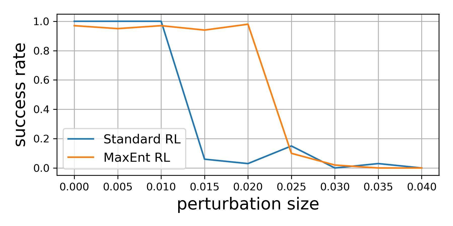
Our theoretical results suggest that, even if we optimize the environment perturbations so the agent does as poorly as possible, MaxEnt RL policies will still be robust. To demonstrate this capability, we trained both standard RL and MaxEnt RL on a peg insertion task shown below. During evaluation, we changed the position of the hole to try to make each policy fail. If we only moved the hole position a little bit ($\le$ 1 cm), both policies always solved the task. However, if we moved the hole position up to 2cm, the policy learned by standard RL almost never succeeded in inserting the peg, while the MaxEnt RL policy succeeded in 95% of trials. This experiment validates our theoretical findings that MaxEnt really is robust to (bounded) adversarial disturbances in the environment.

|

|
|
|
Standard RL |
MaxEnt RL |
Evaluation on adversarial perturbations |
MaxEnt RL is robust to adversarial perturbations of the hole (where the robot
inserts the peg).
Conclusion
In summary, our paper shows that a commonly-used type of RL algorithm, MaxEnt RL, is already solving a robust RL problem. We do not claim that MaxEnt RL will outperform purpose-designed robust RL algorithms. However, the striking simplicity of MaxEnt RL compared with other robust RL algorithms suggests that it may be an appealing alternative to practitioners hoping to equip their RL policies with an ounce of robustness.
Acknowledgements
Thanks to Gokul Swamy, Diba Ghosh, Colin Li, and Sergey Levine for feedback on drafts of this post, and to Chloe Hsu and Daniel Seita for help with the blog.
This post is based on the following paper:
tags: c-Research-Innovation, Manipulation
